Understanding whether a variable’s missingness from a dataset is related to the underlying value of the data is a key concept in the field of missing data analysis. We distinguish three broad categories: missing completely at random (MCAR), missing at random (MAR), and missing not at random (MNAR). In his book Statistical Rethinking, McElreath1 gives an amusing example to illustrate this concept: he considers variants of a dog eating homework and how the dog chooses - if at all - to eat the homework. The examples he give show substantial shifts in observed values, which make for a good illustration of the types of problems you might encounter. A lecture corresponding to the example from the book can be found on YouTube. In this post, I will first briefly review the different missing data mechanisms before implementing McElreath’s examples in SAS.
Overview of Missing Data Mechanisms
My presentation here follows van Buuren2. Let $Y$ be a $n \times p$ matrix representing a sample of $p$ variables for $n$ units of the sample and $R$ be a corresponding $n \times p$ indicator matrix, so that
$$r_{i,j} = \begin{cases} 1 & y_{i,j} \text{ is observed} \\ 0 & y_{i,j} \text{ not observed.}\end{cases} $$
We denote the observed data by $Y_\text{obs}$ and the missing data that $Y_\text{miss}$ so that $Y=(Y_\text{obs},Y_\text{miss})$.
We distinguish three main categories for how the distribution of $R$ may depend on $Y$. This relationship is described as the missing data model. Let $\psi$ contain the parameters of this model. The general expression of the missing data model is $\mathrm{Pr}(R|Y_\text{obs}, Y_\text{miss}, \psi)$, where $\psi$ consists of the parameters of the missing data model.
Missing Completely at Random (MCAR). This implies that the cause of the missing data is unrelated to the data itself. In this case,
$$ \mathrm{Pr}(R=0| Y_\text{obs}, Y_\text{miss}, \psi) = \mathrm{Pr}(R=0|\psi).$$
This is the ideal case, but unfortunately rare in practice. Many researchers implicitly assume this when using methods such as list-wise deletion, otherwise known as complete case analysis, which can produce unbiased estimates of sample means if the data are MCAR, although the reported standard error will be too large.
Missing at Random (MAR). Missingness is the same within groups defined by the observed data, so that
$$ \mathrm{Pr}(R=0| Y_\text{obs}, Y_\text{miss}, \psi) = \mathrm{Pr}(R=0|Y_\text{obs},\psi).$$
This is a often a more reasonable assumption in practice and the starting point for modern missing data methods.
Missing not at Random (MNAR). If neither the MCAR or MAR assumptions hold, then we may find that missingness depends on the missing data itself, in which case there is no simplification and $$ \mathrm{Pr}(R=0| Y_\text{obs}, Y_\text{miss}, \psi) = \mathrm{Pr}(R=0| Y_\text{obs}, Y_\text{miss}, \psi).$$
As you can imagine, this is the most tricky case to deal with.
Dogs Eating Homework
Consider dogs (D) eating students’ homework. Each student’s homework score (H) is graded on a 10-point scale and each student’s score varies in proportion to how much they study (S). We assume the amount of time they study is normally distributed. A binomial is used to generate homework scores from the normed time spent studying. McElreath uses the following code to simulate the full data set:
N <- 100
S <- rnorm( N )
H <- rbinom( N, size=10, inv_logit(S) )
where inv_logit(x) = exp(x)+(1+exp(x)), the definition used by the LOGISTIC function in SAS. With a data step, this can be represented in SAS as follows:
data full;
    DO i=1 to 100;
        S=RAND('NORM');
        H=RAND('BINO', LOGISTIC(S), 10);
        output;
    END;
    label S='Amount of Studying' H='Homework Score';
    drop i;
run;
We can get closer in form to the R code by using PROC IML, but that’s a story for a different post.
Say we are interested in estimating the relationship between $S$ and $H$. In our example, we assume that $H$ is not directly observable. Instead, $H^*$ is observed - a subset of the full data set $H$ with some homework values missing. We can now look at why some of those values are missing. Specifically, in McElreath’s example each student has a dog $D$ and sometimes the dog eats the homework. But here we can again ask, why is the dog eating the homework? McElreath uses directed acyclic graphs (DAGs) to represent different missing data models, reproduced below. As we will see, these are some intuitive examples for our three missing data mechanism categories.
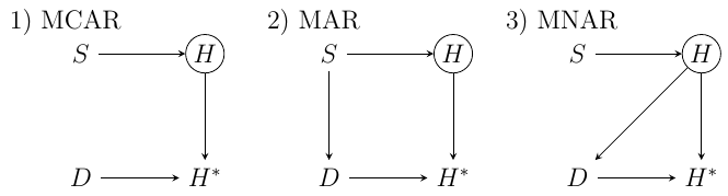
The directed acyclic graphs corresponding to McElreath’s examples of missing data models. $S$ represents the amount of time spent studying, which in turn influences the homework score $H$, which is only partially observed (indicated by the circle). Alas, dogs $D$ eat some of the homework. The actually observed scores - those not eaten - are indicated by $H^*$. Adapted from figure 15.4 in Statistical Rehinking.
Missing Completely At Random (MCAR)
In the first example, the dogs eat homework completely at random. This is the most basic and benign case, and corresponds to DAG 1) in Figure 1. McElreath’s R code is given by
D <- rbern( N )
Hm <- H  # H*, but * is not a valid char for varnames in R
Hm[D==1] <- NA
We can implement this in SAS by using the RAND function with the Bernoulli argument in an if/else clause:
if RAND('BERN', 0.5) then Hm = .;
    else Hm = H;
This causes about half of our data to be hidden, but not in a biased way.
Missing at Random (MAR)
In the second example, we assume the amount of time a student spends studying decreases the amount of time they have to play with and exercise their dog. This, in turn, influences whether the homework gets eaten. Or, as McElreath puts it, the “dog eats conditional on the cause of homework.” In his particular example, the homework is eaten whenever a student spends more time studying than the average $S=0$. This corresponds to DAG 2) in Figure 1.
D <- ifelse( S>0 , 1 , 0 )
Hm <- H
Hm[D==1] <-NA
In SAS:
if S>0 then Hm = .;
    else Hm = H;
Missing not at Random (MNAR)
In this case, we have some correspondence between the missing variable’s value and whether or not it is missing from the data set. Here, the “dog eats conditional on the homework itself.” Suppose that dogs prefer to eat bad homework. In such a case, the value of $H$ is directly related to whether or not $H$ is observed in the particular unit or not. His example R code is as follows:
# dogs prefer bad homework
D <- ifelse( H<5 , 1 , 0 )
Hm <- H
Hm[D==1] <- NA
And in SAS:
if H<5 then Hm = .;
    else Hm = H;
The Full SAS Code
We can now build a SAS data set that contains a full copy of the original data set, together with our various examples of missing data mechanisms. I have added a seed to the data step for reproducibility.
data full;
    CALL streaminit( 451 );

    LABEL
        Type = 'Missing Data Mechanism'
        S = 'Amount of Studying'
        H = 'Homework Score'
        Hm = 'Observed Homework Score'
    ;

    DO i=1 to 100;
        TYPE = 'FULL';
        S = RAND('NORM');
        H = RAND('BINO', LOGISTIC(S), 10);
        Hm = H;
        output;

        /* Example 1) MCAR */
        TYPE = 'MCAR';
        if RAND('BERN', 0.5) then Hm = .;
            else Hm = H;
        output;

        /* Example 2) MAR */
        TYPE = 'MAR';
        if S>0 then Hm = .;
            else Hm = H;
        output;

        /* Example 3) MNAR */
        TYPE = 'MNAR';
        if H<5 then Hm = .;
            else Hm = H;
        output;

    END;

    drop i;
run;
You may want to run a PROC SORT or PROC SQL afterwards to group the different categories together, as they will be alternating in this data set.
Results
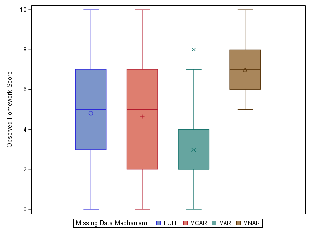
Boxplot of our example data. Note that the MCAR data looks very similar to the original data set, unlike the MAR and MNAR versions.
We can see that MCAR leads to minimal bias in our example data, while both the MAR and MNAR variations lead to substantial differences in observed vs actual homework scores for our synthetic population. For a more subtle example, see section 2.2.4 in van Buuren,2 available online here.