Sampling Regression Lines

Last week we saw how to generate posterior samples using PROC MCMC for simple linear and logistic regression models. This week, I want to show how to sample regression lines from the data set returned by MCMC by plotting several sample regression linse on top of a scatter plot of the source data.

Writing the Macro

Since the majority of the steps are identical irrespective of what data set we use, and because we might want to use this iteretively during model building, I decided to write this up as a macro. To some degree this is required since I will be using a macro do-loop, which is only valid when embedded inside of a macro.

This macro will assume we have fitted a simple linear model of the form

\begin{aligned} y_i &\sim \mathrm{Normal}(\mu_i, \sigma) \\
\mu_i &= \beta_0 + \beta_1 x_i \end{aligned}

Step 1: Get an SRS Sample

The first step is the simplest - selecting a subset of the posterior samples. This is easily achieved by calling PROC SURVEYSELECT.

proc surveyselect data=&posterior. method=srs n=&n.
                  out=SRS;
run;

Step 2: Make a Macro List of Parameters

Next we need to generate a list of intercepts and slopes. I find it easiest to read those in PROC SQL using the into operation. Additionally, we’ll also collect the $x$- and $y$-ranges of our data. This will be used to make sure our plot is centered on the scatter-plot values of our source data set.

proc sql noprint;
  select beta0, beta1 
  into :intercepts separated by ' ',
       :slopes  separated by ' '
  from SRS;

  select min(x), max(x),
         min(y), max(y)
  into :minx, :maxx,
       :miny, :maxy
  from &ds.;
quit;

Step 3: Macro-Loop to Add Lines to a Scatter Plot

Now all the parts have been assembled and you can call PROC SGPLOT. We use the scatter statement to create a scatter plot of the source data. Then we use a do-loop to iteratively paste different lineparm statements corresponding to our different samples into the SGPLOT statement. Lastly, use the xaxis and yaxis statements to focus the graph on the scatter plot data, and not forcing the x-intercepts of the different fitted lines into

proc sgplot data=&ds. noautolegend;
  scatter x=x y=y;
  %do i = 1 %to &n.;
    lineparm x=0 y=%scan(&intercepts, &i, ' ') 
         slope=%scan(&slopes, &i, ' ') / transparency=0.7;
  %end;

  xaxis min=&minx. max=&maxx.;
  yaxis min=&miny. max=&maxy.;
run;

Calling the Macro

And that’s it. Assuming we declared the macro as follows

%macro sample_regression(ds=, posterior=, n=);

we can now call it.

As a particular example, let’s run PROC MCMC’s getting started example 1 straight from GitHub:

filename url gs1 'https://raw.githubusercontent.com/sassoftware/doc-supplement-statug/main/Examples/m-n/mcmcgs1.sas';
%include gs1;

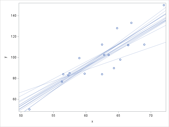
In this example, we predict weight based on height in the sashelp.class data set. The posterior samples are available as work.classout. We’ll want to rename the height and weight variables to $x$ and $y$ in order to work with the chosen macro names. This is easily accomplished by using the rename statement in the macro call itself. We’ll call it with $n=15$.

%sample_regression(ds=sashelp.class(rename=(Height=x Weight=y)),
                  posterior=work.classout,
                  n=15);

This will produce the following output:

With slight modifications you can also use this macro to help you refine your priors. By using the

model general(0);

statement in PROC MCMC in lieu of a regular model you will get estimates of the prior parameters. See the documentation for examples.