In a previous post, I have shown how to connect to the Census API and load data with Python. In this post, I will do the same using SAS instead. Before we get started, two important links from last time: a guide to the API can be found here and a list of the available data sets can be accessed here.
Picking the Data
For this post, I’ll use the same data as last time. There we used the 2018 American Community Survey 1-Year Detailed Table and asked for three variables - total population, household income, and median monthly cost for Alamance and Orange counties in North Carolina (FIPS codes 37001 and 37135). The variable names are not very intuitive, so I highly recommend starting your code with a comment section that includes a markdown-style table of the variables that you want to use. Here is an example table for our data:
| Variable | Label |
|---|---|
| B01003_001E | Total Population |
| B19001_001E | Household Income (12 Month) |
| B25105_001E | Median Monthly Housing Cost |
Building the Query
The next step is to build the query. Like last time, the API consists of a base
URL that points us to the data set we are looking for, a list of the variables
we want to request, and a description of the geography for which we want to
request those variables. Just like last time, I’ll build the query using several
macros for flexibility purposes. Note that since & has a special meaning in SAS,
we need to use %str(&) when referring to it to avoid having the log clobbered with
warnings about unresolved macros.
%let baseurl=https://api.census.gov/data/2018/acs/acs1;
%let varlist=NAME,B01003_001E,B19001_001E,B25105_001E;
%let geolist=for=county:001,135%str(&)in=state:37;
%let fullurl=&baseurl.?get=&varlist.%str(&)&geolist.;
%put &=fullurl;
Your log should now show the full query URL:
FULLURL=https://api.census.gov/data/2018/acs/acs1?get=NAME,B01003_001E,B19001_001E,B25105_001E&for=county:001,135&in=state:37
Making the API Request
The API call is achieved with a simple PROC HTTP call using a temporary file to hold the response from the server.
filename response temp;

proc http url="&fullurl." method="GET" out=response;
run;
Handling the JSON Response
We read the JSON response by utilizing the LIBNAME JSON Engine in SAS.
libname manual JSON fileref=response;
Now run proc datasets lib=manual; quit;. You’ll see two data sets that were created: ALLDATA which contains the whole JSON file’s contents
in a single data set, and ROOT which is a data set of all the root-level data. The latter one is the one we want. Here’s what the
first few observations in each look like:
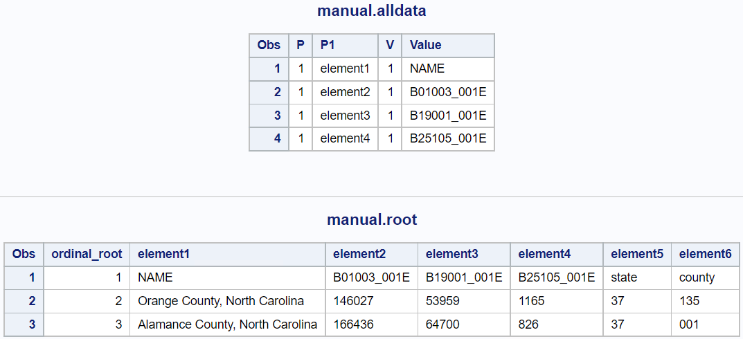
First few observations in the automatically created data sets.
Just like with Python, all columns are treated as character variables at first. Because of the way the Census API is structured, the first row consists of headers, which SAS didn’t use. This is something we’ll need to fix. At this point we have two main routes we can use to fix these issues - we can manually create a new data set from ROOT with PROC SQL and address the issues in that way, or we can take advantage of SAS’ JSON map feature to define how we want to load the JSON when the LIBNAME statement is executed. There are good use cases for each, so I will show both methods.
Cleaning up via PROC SQL
Using PROC SQL, you can rename all the character variables you want to keep. To change from character to numeric,
you’ll use the input function. You can then assign formats and labels as desired. To get rid of the first row,
you can just add a conditional having ordinal_root ne 1 to avoid loading that line.
proc sql;
	create table census as
	select
		element1 as Name,
		input(element2, best12.) as B01003_001E format=COMMA12.  label='Total Population',
		input(element3, best12.) as B19001_001E format=DOLLAR12. label='Household Income (12 Month)',
		input(element4, best12.) as B25105_001E format=DOLLAR12. label='Median Monthly Housing Cost',
		element5 as state,
		element6 as county
	from manual.root
	having ordinal_root ne 1;
quit;
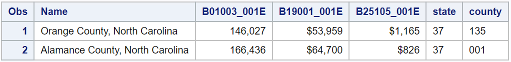
Result from the PROC SQL method.
A benefit of this method is that as you fix the input table, you can already begin to work with
it thanks to the calculated keyword in PROC SQL. Say we weren’t actually interested in housing cost and
household income, but instead would like to know what percent of their annual income a household spends on
housing in a given county. We could just add a new variable to our PROC SQL call and build our table like this:
proc sql;
	create table census as
	select
		element1 as Name,
		input(element2, best12.) as B01003_001E format=COMMA12. label='Total Population',
		input(element3, best12.) as B19001_001E format=DOLLAR12. label='Household Income (12 Month)',
		input(element4, best12.) as B25105_001E format=DOLLAR12. label='Median Monthly Housing Cost',
		/* Now calculate what we want from the new columns: */
		12*(calculated B25105_001E)/calculated B19001_001E as HousingCostPCT format=PERCENT10.2,
		element5 as state,
		element6 as county
	from manual.root
	having ordinal_root ne 1;
quit;
Using a JSON MAP
Alternatively, we could change the way SAS reads the JSON data by editing the JSON map it uses to decode the JSON file. The first step is to ask SAS to create a map for us to edit:
filename automap "sas.map";
libname autodata JSON fileref=response map=automap automap=create;
The map will look something like this: Beginning of the automatically created JSON map.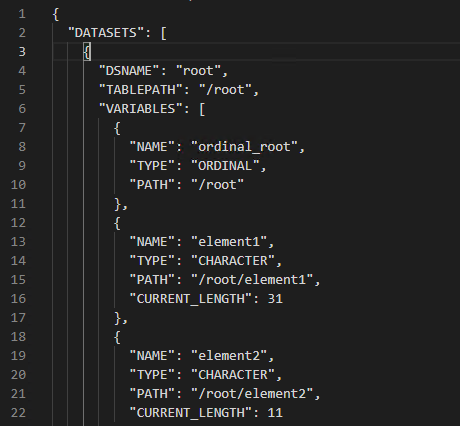
Note that this is also a JSON file which you can edit in a text editor. With this map, you can change the names
of the data sets and variables, assign labels and formats, and also re-format incoming data. Variables and data sets
you don’t want to read can simply be deleted from the map. Here’s the beginning of my edited file: Beginning of my edited JSON map.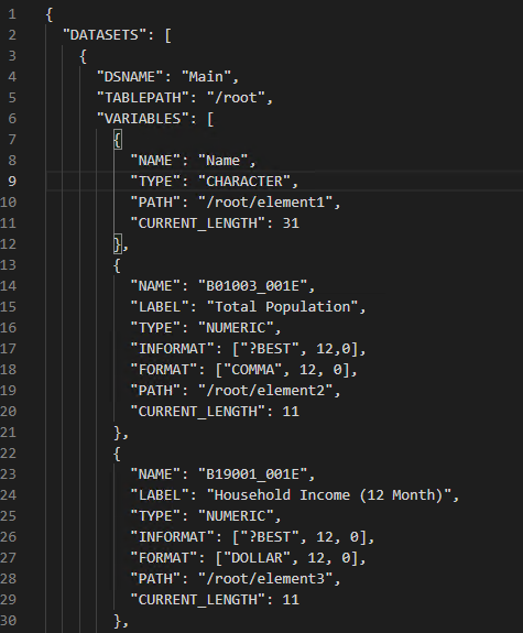
Since the first row of observations in the JSON are actually a header and non-numeric, I add ? prior to the
specified informat. This prevents errors in the log and simply replaces non-matching variables with missing values.
We can now reload the JSON using our custom map by dropping the automap=create option from the LIBNAME statement:
libname autodata JSON fileref=response map=automap;
When I now print the resulting data set, the header row is still there, but replaced by missing values in numeric
columns: The data set as a result of the edited JSON map.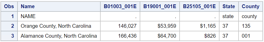
This means we’ll need to additionally drop this row in a separate step using a delete statement either in a PROC SQL or DATA step.
Whichever method you choose, you now can access data via an API call from SAS. Happy exploring!