CMSRP
Data Analytics Workshop
by Michael Senter, PhD
2023-06-02
What is our Goal Today?
- Discuss challenges you may face.
- Get the right vocabulary to make decisions this summer.

Ask questions!
Foundations
Statistics is Hard
The Boy-or-Girl Paradox
Mr. Smith says, “I have two children and at least one of them is a boy.”
What is the probability that the other child is a boy?
Gardner, M. (1961). The 2nd Scientific American Book of Mathematical Puzzles and Diversions. New York, NY: Simon and Schuster.
What do you think?
Mr. Smith has two children and at least one of them is a boy. Then the probability that the other child is a boy is...
- \(1/2\)
- \(1/3\)
- \(1/4\)
- \(2/3\)
- Other
Solution - Count the Paths!
"Mr. Smith has two children and at least one of them is a boy"

The key is to realize we don't know which child is the boy - the first or the second.
Example - Intepreting Regression Results
| Gender | Ethnicity | Year | |
|---|---|---|---|
| BMI ≥ 25 | All | All | 2048 |
| Men | All | 2051 | |
| Non-Hisp. White | 2049 | ||
| Non-Hisp. Black | 2095 | ||
| Women | All | 2044 |
Year when prevalence of overweight and obese individuals in US reaches 100% in linear regression model. Adapted from Wang et al (2008), DOI: 10.1038/oby.2008.351.
Form of Basic Linear Regression
\[\begin{aligned} y_i &\sim \mathrm{Normal}(\mu_i, \sigma) \\ \mu_i &= \beta_0 + \beta_1 x_i \end{aligned}\]The distribution of $\beta_0$, $\beta_1$, $\sigma$ to be determined.
Linear Regression - Concrete Example 1
\[\begin{aligned} \mathrm{height}_i &\sim \mathrm{Normal}(\mu_i, \sigma) \\ \mu_i &= \beta_0 + \beta_1 \, \mathrm{weight}_i \end{aligned}\]For adults, height and weight are approximately linearly related.
Linear Regression - Concrete Example 2
Wang et al (2008)
\[\begin{aligned} \mathrm{bmi}_i &\sim \mathrm{Normal}(\mu_i, \sigma) \\ \mu_i &= \beta_0 + \beta_1 \, \mathrm{time}_i \end{aligned}\]Use the whole data set, then rinse & repeat with different subsets.
Foundations
Be Wary of Point Estimates
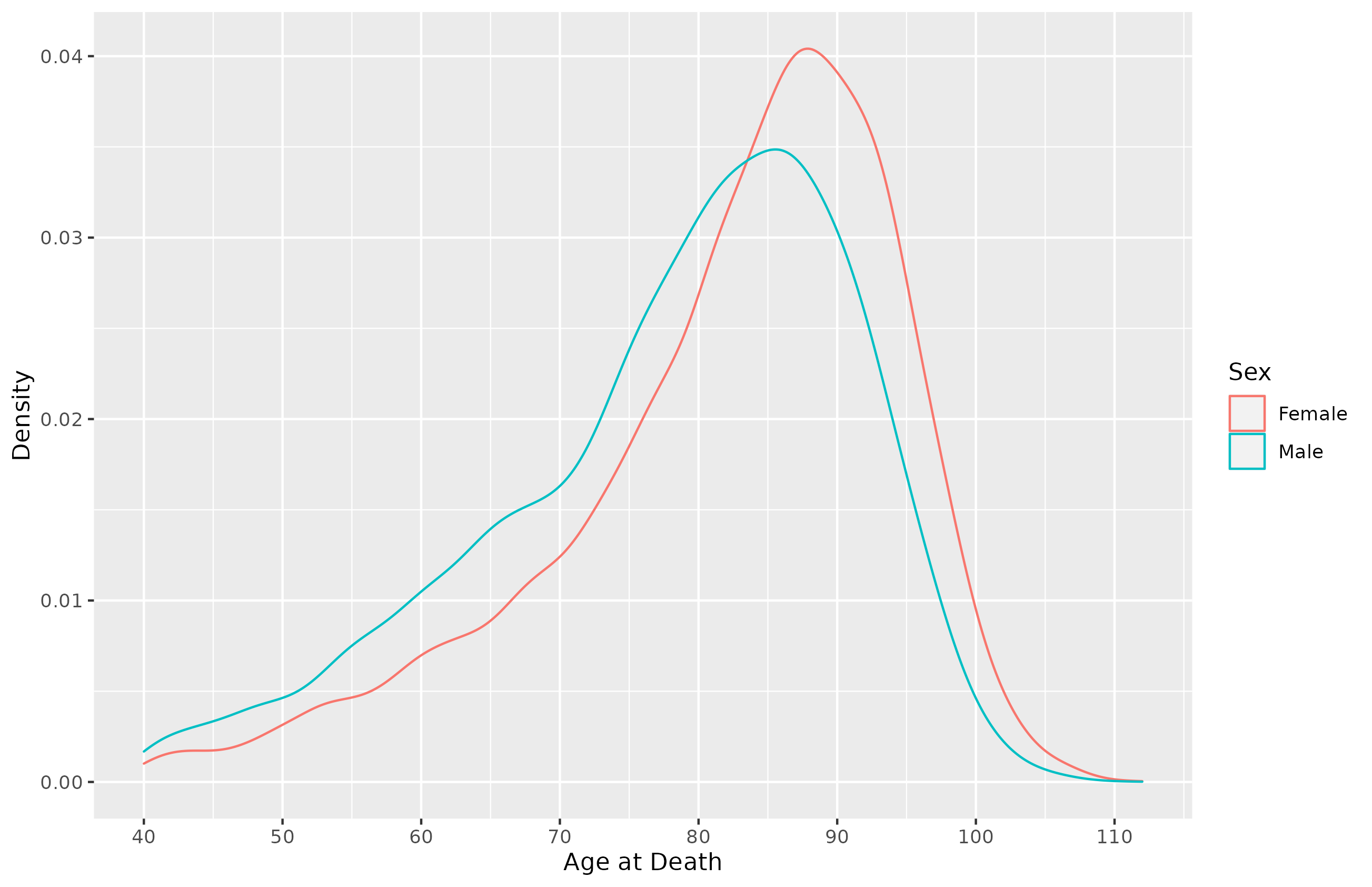
Life Expectancy
Question 1: What is expected age of death for a 40 year old?
Answer 1: 76.97 for Males, 81.38 for Females.
Question 2: What is the median age of death for a 40 year old?
Answer 2: 81 for Males, 85 for Females.
Source: SSA Mortality Table, 2020.
Consider the Actual Distribution of Deaths
Foundations
Ignore Significance Tests
Null hypothesis Significance Testing
Meaning of Terms
- Null-hypothesis $\coloneqq$ "no effect/difference"
- This is essentially never true in real life.
- Significance Test $\coloneqq$ "if the null hypothesis were true, how probable is a result at least as extreme as my result?"
- Doesn't actually say anything about your research hypothesis, only about the null hypothesis that you don't believe in to begin with.
Significance Tests Sensitive to Sample Size
Population
\[\begin{aligned} \mu &= 100 \\ \sigma &= 15 \end{aligned}\]Sample
\[\begin{aligned} \bar{x} &= 102 \\ n &= \text{ varies} \end{aligned}\]Z-Score Test
\[\begin{aligned} z = \frac{\bar{x}-\mu}{\sigma / \sqrt{n}} \htmlClass{fragment}{=\frac{\bar{x}-\mu}{\sigma} \sqrt{n}} \end{aligned}\]Minimal Sample Size for P-Value
| P-Value | Z-Score | N |
|---|---|---|
| 0.05 | 1.645 | 153 |
| 0.025 | 1.960 | 217 |
| 0.01 | 2.326 | 305 |
Doesn't answer the question whether the difference $\bar{x}-\mu $ actually matters clinically.
Do you think it matters how big \(|\bar{x}-\mu|/\sigma_x\) is?
Beware of False Conclusions!
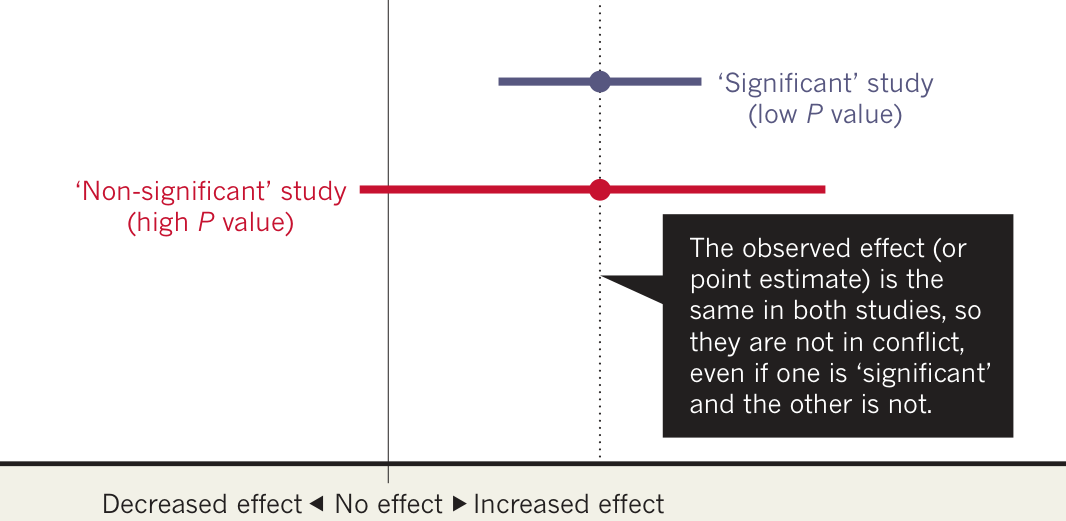
More on P-Values
- The P-value depends on the sample size/space.
- The P-value is not the probablity that \(H_0\) is (not) true.
- The P-value depends on fictive data.
- The P-value is not an absolute measure.
- The P-value does not take all evidence into account.
- ... and other issues. See chapter 1 in Lesaffre and Lawson (2012) for an accessible discussion.
Some Worthwhile Reading
- Amrhein, V., Greenland, S., and McShane, B. (2019), “Scientists rise up against statistical significance,” Nature, 567, 305–307. DOI: 10.1038/d41586-019-00857-9.
- Gelman, A. (2013), “Misunderstanding the p-value,” StatModeling blog.
- Gelman, A. (2018), “The failure of null hypothesis significance testing when studying incremental changes, and what to do about it,” Personality and Social Psychology Bulletin, 44, 16–23. DOI: 10.1177/0146167217729162.
- Gelman, A. (2019), “Thinking about "Abandon statistical significance," p-values, etc.,” StatModeling Blog.
Reproducibility
Keep All Your Materials Together
Organization
Keep your data, code, and analysis all in one folder. This helps with
- Organization: no need to search all over for different components of your research project.
- Backups: archive a single folder to ensure your work is not lost.
- Reproducibility: others can reliably follow your steps, even years later.
Suggested Folder Structure
                    $ exa --tree cmsrp-project-23/
                    cmsrp-project-23
                    ├── data
                    │  ├── alternative-subset.csv
                    │  └── cmsrp-project-data.csv
                    ├── data-dictionary.csv
                    ├── docs
                    │  ├── abstraction-protocol.docx
                    │  ├── aca-24-abstract.docx
                    │  ├── bibliography.bib
                    │  └── irb.pdf
                    ├── raw_data
                    │  └── 2023-06-01-redcap.csv
                    ├── README.md
                    └── scripts
                        ├── analysis.sas
                        ├── data_transform_validation.sas
                        └── load_raw_data.sas
Use an archiving program like zip or 7z to share/backup all or parts of your project. If your project includes PHI, there is a minimum encryption standard (AES-128).
Use Version Control
- Keeps track of who changed what, when, and why.
- Makes changes reversible.
- Works best with text-based data.
- Available as part of REDCap or manually via Git.
On that note: Don't send multiple versions of a word doc around as you edit. This leads to many problems. Use OneDrive instead.
Reproducibility
Use Science to Guide Variable Selection
Big Picture - Scientific Process
- Define the estimand(s) of interest.
- Create scientific model(s).
- Create statistical model(s).
- Analyze your models.
Define Your Estimand
- Be specific. Example attributes:
- Treatment condition of interest (clinical trial).
- Patient Population.
- Variable to be obtained.
- For details, review ICH E9 (R1) addendum on estimands.
- Pay attention to the difference between what you want to know and what you can measure.
Your choice of estimand alters how your study is properly interpreted.
Scientific Model ≠ Statistical Model

Hypotheses do not imply unique models,
and models do not imply unique hypotheses.
No causes in - no causes out
Statistical Inference
≠
Prediction
≠
Causal Analysis
If you want to make any causal statements, you need to carefully consider the assumed causal model.
Introduction to DAGs
- DAG - "Directed Acyclical Graph."
- Represents the qualitative aspect of the data generating process: \(X \rightarrow Y\).
- Three main building blocks:
- Mediators
- Common Cause (forks)
- Common Effects (colliders)
The Mediator

$X$ causally affects $Y$ through mediator $Z$.
Conditioning on $Z$ blocks the association.
The Common Cause (Fork)

$X$ and $Y$ share a common cause (confounder) $Z$, leading to a non-causal association between both.
Conditioning on $Z$ blocks this association.
Common Effects (Collider)

There is no association between $X$ and $Y$.
If you condition on $Z$, you introduce a non-causal association between $X$ and $Y$.
What's the point?
Depending on what variables you use as covariates, you may either induce or obscure a causal relationship. Either way, your interpretation of the coefficients will be incorrect.
Don't do a "garbage-can" regression (see Achen 2005).
Example: The Birth-Weight Paradox
- Low birth weight is a strong predictor of infant mortality.
- Infants born to smoking mothers have lower birth weights on average.
- Low birth weight infants born to smoking mothers have a lower infant mortality rate than those born to non-smoking mothers.
Is smoking beneficial, protecting low birth weight infants against infant mortality?
Example: The Birth-Weight Paradox
- $n=4\,115\,494$ infants born in USA in 1991. For $3\, 001\,621$ infants born, maternal smoking status is known.
- Mean birth weight: $3\,145$ g (smokers) vs. $3\,370$ g (non-smokers).
- Unadjusted infant mortality rate ratio: 1.55.
- Infant mortality rate ratio, adjusted for birth weight: 1.09.
- LBW infant mortality rate ratio, adjusted for birth weight: 0.79.
See DOI 10.1093/aje/kwj275 for details.
Consider the DAG


Stratifying by birth weight introduces a spurious association between smoking and mortality.
See DOI 10.1093/aje/kwj275 for details.
What do I do about it?
- Construct a DAG reflecting your model.
- Use software to help you pick appropriate covariates given your model.
- SAS: CAUSALGRAPH procedure.
- R: DAGitty.
- To understand the way this works, read Cinelli, Forney, and Pearl (2020).
Build A DAG

Start with your research question.
Build A DAG

Add treatment, outcome, and mediators to your DAG.
Build A DAG

Start adding common causes to outcome...
Build A DAG

... and treatment. Ignore most exogenous error terms.
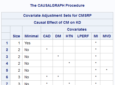
Example DAG - Code
                    proc causalgraph;
                        model "CMSRP"
                            HTN => CM, CM => LPERF, LPERF => KD,
                            DM => MVD, MVD => LPERF KD,
                            CAD => MI, MI => CM KD;
                        IDENTIFY  CM => KD;
                    run;
Example DAG - SAS Output
Pro-Tip:
Try Simulating Assumptions
- Use your statistical model to simulate fake data.
- Some benefits:
- Clarifies what your model implies. How big should an effect be, etc.
- Allows for repeat sampling, so you can see how your model behaves.
- Provides an opportunity to debug your analysis code.
Reproducibility
Have a Codebook
What's a Codebook?
- Gives a summary of what your project is about.
- Defines variable names, their meaning, units, and possible values.
- Ideally has a machine-readable component.
- If you use REDCap, it can generate this for you.
Variable Naming
- Variable Names should be consistent and predictable.
- Treatment and control data should be in the same data set.
- Then how do I distinguish between the treatment and control?
- Use a "dummy variable."
What is a dummy Variable?
A dummy variable takes either the value 0 or 1 and can be used to show group membership. Example:
| Treatment | Subject | Month | Serum Cholesterol (mg/dL) |
|---|---|---|---|
| 1 | 1 | 0 | 178 |
| 1 | 1 | 24 | 274 |
| 0 | 63 | 0 | 251 |
| 0 | 63 | 24 | 248 |
Categorical Variables
Collect these as integers, not as strings. Use dummy or index variables.
Example:
| Bad Scheme | Good Scheme | |
| Gender | Male | 0 |
| Female | 1 | |
| BMI | Normal | 1 |
| Overweight | 2 | |
| Obese | 3 |
Why not just use Text?
- Typing in a string is error prone. The computer treats 'y', 'Y', 'Yes', and 'yes' each as a distinct option, even if that's not what you mean.
- Statistical Software needs to convert strings to numbers to work, anyways. Consider this ahead of time.
- Dummy/indicator and index encodings work well for most use cases. Other options exist, but prefer to recode in analysis step over using those encodings directly in your data set.
Data Collection
Have an Abstraction Protocol
Define how you will collect your data.
- Where will you get the information from?
- How will the source information be mapped to your codebook?
- If you search medical records, what search terms will you use? Record every variant you will be using.
- This protocol needs to be in writing.
- Follow this religiously. Deviations kill reproducibility and make your study arbitrary. Don't be arbitrary.
How to store your Data?
- Don't use Excel sheets.
- Consider using REDCap.
- Widely used database software in medical research.
- Helps you build a codebook that is used to validate data as it is entered, preventing mistakes.
- Convenient export to statistical software such as SAS or R.
- Provides tracking of changes.
- CSV Files.
- Software agnostic.
- Could be read 30 years ago, can still be read 30 years from now.
- Can provide tracking if used with version control.
- Requires manual data validation.
Automate What You Can
- Will you remember your choices and methods exactly, even 5 years from now?
- The more you do by hand, the less reproducible your study becomes.
- Computers do exactly what you tell them to, every time. But you might make typos.
- Let computers handle as much of tedious tasks as possible. E.g.,
- REDCap forms for data entry.
- Scripts to automate data acquisition and formatting.
Validation and Completion
Check Your Data
- Load everything in your software of choice.
- Is everything formatted correctly?
- Make plenty of graphs.
- If necessary, apply fixes using scripts to any formatting issues. Don't do this by hand!
- If you have missing observations, check your source docs to see if they were overlooked during abstraction.
What about Missing Data?
- You probably will have missing data. That's ok.
- In what way the data is missing will impact results and analysis.
- Missing Completely at Random (MCAR)
- Missing at Random (MAR)
- Missing not at Random (MNAR)
- Key difficulty: the data itself cannot show you which mechanism is applicable in your case. But you need to know which mechanism applies to interpret the analysis correctly.
Missingness Mechanisms Have Important Effect
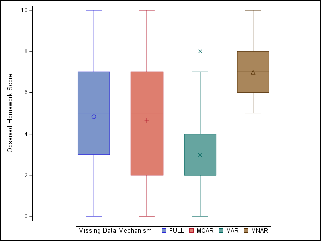
See here for example details.
Some Ad-Hoc Methods
- Complete Case Analysis (CCA)/Listwise deletion
- Pairwise deletion
- Mean imputation
- Regression imputation
Assumptions by Ad-Hoc Methods
| Mean | Reg Weight | Standard Error | |
| Listwise | MCAR | MCAR | Too Large |
| Pairwise | MCAR | MCAR | Complicated |
| Mean | MCAR | - | Too small |
| Regression | MAR | MAR (y) | Too small |
These methods not general enough. Multiple imputation is better.
Adapted from van Buuren (2018).
Multiple Imputation - Basic Idea
- Generate multiple copies of the data set with missing values drawn from a specified distribution.
- Analyze each of these (now complete) data sets using standard methods.
- Combine the results using Rubin's rules.
Software can do this for you, but this can still be difficult for newcomers. For a gentle introduction, try Schafer (1999) or van Buuren (2018).
Basic Reporting Guidelines
- How much data is missing? How many complete observations do you have?
- Reasons for missingness?
- What are the consequences?
- What are your methods and assumptions?
See section 12.2 in van Buuren (2018) for more details.
Recommended Reading
Doing Statistical Modeling

YouTube Lecture Playlist
Recommended Reading
Consuming Statistical Models


Some Resources
- ITS Virtual Lab: Access to software like SAS, Stata, etc.
- REDCap Database
- Low/no-fee services to help with REDCap available at NC TraCS.
- General tutorials available from Project REDCap
- NC TraCS databases: Partnership with RTI and others. Includes insurance data, hospitalization data, cancer databases, maternal and neonatal health, etc.